Inventory Forecasting with AI #6

Inventory Forecasting with AI

6. Outliers in the Data – The Next Step Toward Robust Forecasting

Why Handle outliers?

Every product range occasionally experiences a one-time “spike” – for example, a customer purchasing hundreds of units for their own promotion, or a company buying out an entire truckload. These volumes are real, but non-repeatable, and they stand out significantly during a typical month.

How will the model react?

The model overfits to the extreme – begins to overstock an item that normally sells only in small quantities.
The model ignores the extreme – learns that the spike is just noise, and in the process, suppresses real seasonal peaks.
The model shares patterns across products – a single outlier can disrupt entire product groups.
Large absolute errors inflate evaluation metrics (e.g., RMSE).

The chart shows detected outliers across the full dataset. It’s clear that even with a high detection threshold, many outliers exist and deviate significantly from the average.
That’s why outlier detection is necessary and decide what to do with them. The key question is: Where does legitimate sales volume end, and an outlier begin?

Note: At standard detection settings, we’re already seeing over 1,000 outliers.

How Do I Detect Outliers?

I use a combination of a robust center (trimmed mean), MAD-score, and percentile-based filtering. Sales values that are both above the x-th percentile and further than k × MAD from the center are labeled as outliers and capped to a “safe upper limit”.

MAD-score: |x – median| / MAD
MAD = median absolute deviation

Threshold Options:

No outliner cut – Keep all extremes
Medium outliner cut (threshold k ≈ 3–4) – Model becomes more stable, but we risk removing valid seasonal peaks
Top outliner cut (threshold k ≈ 8–10) – Keeps most of the data, filters only true outliers; in testing, this proved to be the safest compromise

Striking a Balance

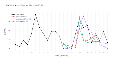
Outlier handling is a nuanced topic. According to metrics, a “medium cut” delivers the best results. However, this setting trims thousands of peaks — including some that may represent real demand — and can ultimately backfire.

Metrics	No outliner cut		Medium outliner cut		Top outliner cut
Metrics	Value (ALL)	Value (Item)	Value (ALL)	Value (Item)	Value (ALL)	Value (Item)
WAPE	30.2608	44.5829	28.8406	42.9816	28.7899	43.5887
RMSE	46.1427	22.3537	48.0208	21.3234	48.2553	21.7787
R²	0.9012		0.9141		0.8904
MAPE	60.0505		58.8268		56.4778
ROBUST	0.4948	62.2027	0.5001	61.8983	0.4874	62.6898
STABLE	0.365		0.3482		0.3718

My decision:
After visual inspection, I decided for a conservative approach — cut only the most extreme spikes. This way, the model retains important seasonal signals. The metrics may lose a bit of precision, but the forecasts stay more faithful to real product behavior.

I’d rather accept a WAPE point increase than risk chopping off half of the Christmas demand.

Sparse Categories

Besides turnover outliers, another problem emerges: categories with very few items.

Why is this harmful to the model?

During deep learning training, each category gets an embedding vector (which encodes similarities between categories). For a group with only a handful of items, the vector is trained on virtually no data:

It carries no meaningful signal (the network doesn’t “learn” it)
It dilutes model capacity – adding parameters that don’t contribute to prediction
It increases the risk of overfitting to that single item

Solution:

Merge all sparse segments into a single label, e.g. “unknown”.
Keep all other groups with sufficient size unchanged.

This way, embeddings are only created for categories that have at least several items – resulting in fewer but more informative vectors. It also reduces VRAM requirements.

Other settings

Once the data was cleaned and enriched with meaningful features, the second half of the job began — convincing the neural network to learn the right way.
In practice, this is like fine-tuning a coffee machine: same beans, same water, but tiny differences in pressure or temperature make all the difference in taste.

Modern deep learning models have orders of magnitude more parameters than classic algorithms — and dozens of hyperparameters to tune. The final setup always depends on the character of the data (seasonality, promotions, long-tail) and the business goal (minimize stockouts, reduce inventory, estimate uncertainty).

A Few Key Parameters:

Loss Function – what we consider an error
A function that measures the difference between model prediction and reality, guiding how much the network should adjust during training.
Optimizer – how the model learns
An algorithm that updates neuron weights based on the loss and its gradients to improve predictions.
Learning Rate – how fast the model learns
Controls how much the weights are adjusted at each training step.
Model Size – learning capacity

The number of neurons and layers determines how many patterns the model can absorb.

Summary – Current Progress

At this stage, I wrapped up the preparation phase and ran the first test on scenario #2:

33 months of historical data for training
3 months of validation data, not seen during training
Only items with a complete 36-month history
Feature engineering complete
Extreme values trimmed

Metrics	Value (ALL)	Value (Item)
WAPE	28.4178	42.0787
RMSE	46.3156	21.1877
R²	0.9004
MAPE	52.4587
ROBUST	0.4986	59.7858
STABLE	0.3677

The results confirm that combining enriched features with outlier control delivers the first practically usable outcomes — predictions are more stable and, most importantly, capture both the trend and the absolute demand level more accurately.

However, even after all these improvements, visual inspection revealed three specific types of items where the model still struggles:

Item type	Symptoms	Why It’s a Problem
Seasonal Sales	10 months of zero sales, then a sudden spike	Model smooths the peak as noise
Zero Predictions	Irregular sales, frequent zero months	Forecasts drift toward zero
Promotions	Sales increase only slightly during promos	Promotional effects aren’t reflected properly in predictions

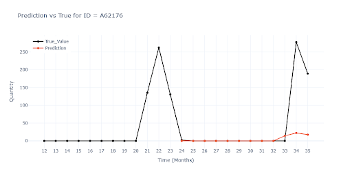
The chart illustrates a typical seasonal item. The model fails to reproduce this seasonality without further support.

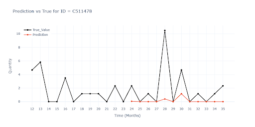
In some cases — mostly low-turnover items with frequent zeros — the model persistently predicted zeros, regardless of past spikes.

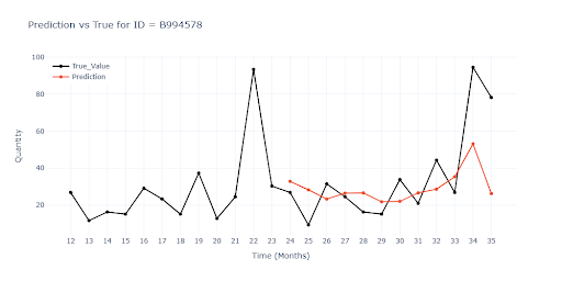
Another graph shows the model’s poor reaction to promotional campaigns. Months 34 and 35 were marked as promotional periods (as in previous years), but the model responded only marginally.