#6. Forecasting in Practice: Technical Perspective

Forecasting in Practice

Technical Perspective

In the previous articles, I focused on the business perspective — when statistical models, machine learning, and deep learning make sense. This article goes one layer deeper. It focuses on how the solution is actually built, what decisions need to be made, and why the model itself represents only a small part of the overall problem.

The goal is not to explain theory, but to show how forecasting experiments are created and evaluated in practice.

Technical Differences Between Approaches

Statistical, machine learning, and deep learning models were not tested as isolated approaches.

All of them operated on the same dataset and used the same data preparation pipeline. The key difference was therefore not the data itself, but the number and complexity of technical decisions required to make the individual approaches work effectively.

For statistical models, the number of such decisions is relatively small — typically involving proper time series preparation, data frequency, and validation horizon.
With machine learning, input features become much more important because the model itself does not inherently understand temporal relationships.
Deep learning introduces another layer of decision-making — handling inputs, normalization strategies, loss functions, and the configuration of the model itself.

Experiment Definition

Each experiment is defined as a combination of independent decisions that can be modified and evaluated separately.
These typically include:

definition of input data
feature engineering
normalization
loss functions
model parameters

Each of these components can be adjusted independently while observing its impact on the results. The goal is not to find one universally optimal configuration, but to understand how individual components influence model behavior.

Input Data

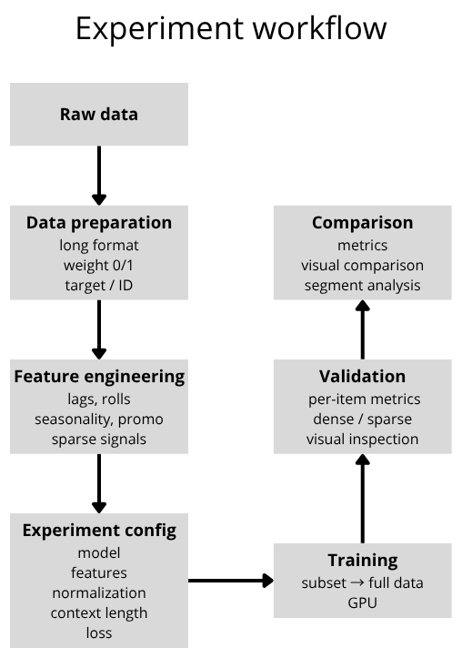
The dataset is prepared in a long-format structure, where each row represents a combination of a specific time step and a particular ID. An important component is the binary weight feature, which indicates whether the product actually existed at a given point in time.

This information is critical because most forecasting frameworks cannot work directly with missing values (NaN). Without explicit differentiation, the model would interpret non-existent historical periods as real observations.

Feature engineering

Feature engineering transforms raw data into signals that the model can learn from. Well-designed features allow the model to capture relationships that are not directly visible in the raw data itself. For complex or irregular datasets, this layer often has a greater impact than the choice of model alone.

It typically includes:

temporal dependencies (lags, rolling statistics)
seasonal and calendar-related information
promotional and campaign indicators
signals designed for sparse data
group-level information
external inputs (when available)

Model Selection

Each experiment is fully defined through configuration. Instead of modifying the code between experiments, only the configuration parameters are changed. This makes it possible to systematically test different combinations and compare them directly against each other.

The configuration typically defines:

the model type
model parameters
the target loss function
input and output sequence lengths (encoder/decoder)
training duration

Each of these components can be modified independently while observing its impact on the results. The experiment is therefore fully described by a configuration that defines both the data processing pipeline and the forecasting model itself.

📋

filename.json

"Experiment TFT 1": {
       "config_def": {
            "TARGET_NORMALIZER" : {"method":"standard", "group":True, "center":True, "transformation":"none"},
            "FEATURE_NORMALIZER": {"method":"default", "group":True, "center":None},
            "LOSS_WEIGHT": {"zero":0.8, "low":1, "normal":1, "high":1},
        },
        "params": {
            "model_name":          	 "TFT",
            "epochs":               	40,
            "batch_size":           	256,
            "optimizer":            	"AdamW",
            "learning_rate":        	1e-3,
            "learning_strategy":    	"plateau",
            "dropout" :             	0.1,
            "hidden_size" :         	128,
            "layers" :         		2,
            "prediction_length":    	prediction_length,
            "encoder_length":       	encoder_length,
            "loss":                 	"QuantileLoss([0.1, 0.3, 0.5, 0.85, 0.95])",
            "gradient_clip_val" :   	0.5,
            "hidden_continuous_size":	8,
        },
        "features": 			list_of_features,
    },
    
    list_of_features=  [
        ("bins_volume",{}),
        ("sell_time_features",{}),
        ("encode_date_harmonics", {"harmonics": [1, 2, 3]}),
        ("discount_action_features",{}),
        ("peak_seasons",{"is_peak":False}),
        ("lag_feature",{"lags":["1M", "1Y", 6]}),
        ("roll_log_feature",{"rolls":["1M", "1Y", "2Y"]}),
        ("trend_Group_feature",{}),
        ("lag_Group_feature",{}),
        ("wavelet_target_group",{}),
    ]

Working with History and Context

Forecasting frameworks generally cannot work directly with missing values (NaN), which makes it necessary to explicitly distinguish between real historical data and contextual information.

For this reason, I use a binary weight feature:

1 — represents real historical data
0 — represents contextual data that does not contribute to the loss calculation

This allows the model to see the complete temporal structure while avoiding penalization for periods that do not correspond to actual historical observations. This is especially important for products with short histories, where a large portion of the timeline contains no real data.

Synthetic Context

Synthetic context is used to extend short time series to the required encoder length. It is generated based on product similarity, using static attributes such as product groups. As a result, the model does not learn only from the limited history of a single product, but also leverages patterns shared across similar products. The same principle applies to embeddings, where new or sparse products are not processed in isolation, but rather within the context of the broader product group.

Experiment Workflow

Experiments are not performed as one-time model training runs, but rather as an iterative process. I typically begin with a smaller subset of the data (hundreds to thousands of IDs), where basic parameter combinations can be tested quickly. Once a promising configuration appears, it is gradually scaled to the full dataset.

Because the entire pipeline is configuration-driven, there is no need to modify the code itself — only the parameters are adjusted while systematically comparing results across different variants.

The entire process is constrained by available computational resources (primarily GPU performance), so experiments are executed sequentially, with each variant utilizing the maximum available compute capacity. Results are evaluated using a combination of automated analysis and manual inspection (primarily through Weights & Biases). The focus is not only on global metrics, but also on performance for specific product categories and on visual analysis of the forecasts themselves.

Validation

Validation is performed on time steps that were not used during training in order to reflect a real forecasting scenario. The evaluation metrics are not calculated globally across the entire dataset. Instead, they are first computed separately for each individual product and only then aggregated.

This approach allows me to:

prevent large-volume products from masking the behavior of smaller ones
verify whether the model performs consistently across the entire portfolio

In addition to average metrics, I also analyze specific time series directly (seasonal, sparse, irregular), because aggregate metrics alone often fail to reveal the actual type of forecasting error.

Dense Metrics (projects 1 and 3)

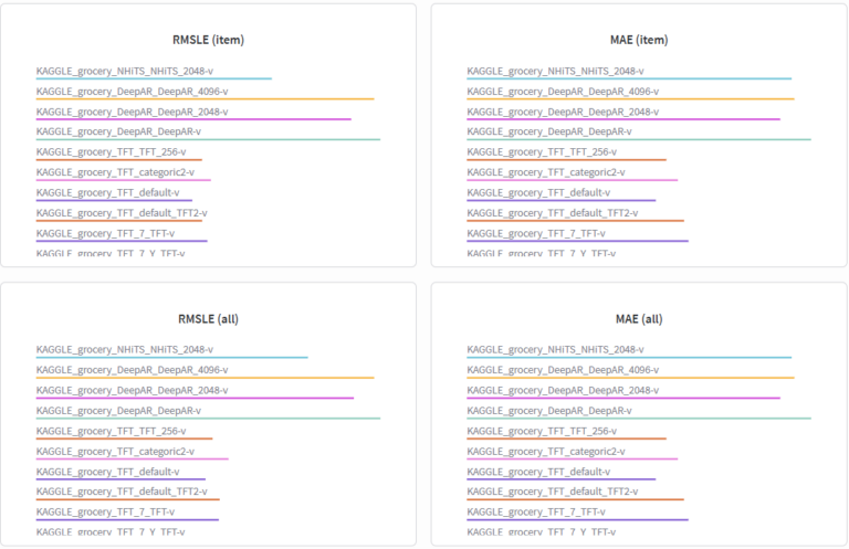
For more stable forecasting scenarios, I primarily evaluate quantity prediction error:

MAE — absolute error measured in target units
RMSLE — relative error with reduced sensitivity to extreme values

I also use modified variants of WAPE for better interpretability, including:

metrics tracking error direction (bias)
metrics limiting the influence of extreme values
metrics focused on the stable part of the portfolio

Intermittent Metrics (project 2)

For sparse-data projects, where a high proportion of zero values strongly affects standard metrics, I use a different approach by separating the problem into two parts:

whether the model correctly identifies the occurrence of a sale (YES/NO)
how accurately it predicts the sales quantity

I therefore use metrics divided according to the type of situation:

metrics for zero-sales periods (ZERO_MAE, ZERO_HIT_RATE)
metrics for positive sales (POSITIVE_WAPE, POSITIVE_MAE)
metrics focused on sales peaks (PEAK_POSITIVE_WAPE)
metrics tracking error direction (SIGNED_BIAS)

The objective is not to optimize a single metric, but to understand model behavior across different types of scenarios.

Conclusion

The final result is a collection of evaluated experiments with fully described configurations that can be easily modified without changing the implementation itself. Individual components — inputs, data representation, normalization, loss functions, or the model architecture — are modified independently while tracking their impact on the results.

The entire series of projects demonstrated that forecast quality is not determined by a single model, a single metric, or one universally “correct” approach. The decisive factor is primarily the nature of the data itself.

Stable datasets with sufficiently long historical data can often be handled very effectively using relatively simple approaches. However, once the data begins to combine short history, irregularity, sparse behavior, seasonality, promotional events, or external influences, the problem becomes significantly more complex — and the differences between individual approaches become much more substantial.

The experiments also showed that the main advantage of deep learning lies in its ability to handle complexity:

combining a large number of input signals
identifying patterns across the entire portfolio
handling irregular and sparse behavior
reacting to changing context over time

One of the conclusions of the entire series is that aggregate metrics alone are not sufficient. Models with similar average results can behave very differently on critical products or during important fluctuations. Forecast evaluation therefore requires not only numerical metrics, but also contextual and visual analysis.

The series also highlighted a practical reality that is often underestimated in discussions about AI forecasting: the biggest challenge is usually not training the model itself, but building a process that allows experiments to be systematically managed, compared, and translated into real business decisions.