Inventory Forecasting with AI
9. Forecasting Short-History Items
Summary
In the previous chapter, I trained the model on the entire assortment for the first time – not only SKUs with a full 36-month history, but also those with just a few months of data, or even no history at all.
- Only items with a full history
- Items with at least one month of history
- The entire dataset, including items with no history at all
The minimum 1 month of history variant delivered the highest stability – the model was able to use as much data as possible without training on “empty” rows. However, detailed validation revealed that the biggest weakness remains items with less than 6 months of history:
- Items with at least 6 months of history are handled relatively reliably.
- Below this threshold – especially for brand-new SKUs – errors increase sharply.
- The most common problem: the model fails to estimate even the basic scale – it doesn’t know whether to forecast 10, 100, or 1,000 units.
Feature Engineering III – Group Features
In chapter five, I showed how additional features can turn raw numbers into a “map” that allows the neural network to orient itself and predict demand with useful accuracy.
This time, however, I’m targeting items with short history, which simply don’t contain enough information for the model to make accurate predictions on their own.
The goal
- Find similar items – those sharing the same category, seasonality, and promotion behavior.
- Use group embeddings – each segment receives its own vector capturing demand similarity.
- Calculate group averages – if an item has no history, the model can use averages from its group.
- Add these values as new features – the network learns that it can “transfer” information from rich series to sparse ones.
Why it works
- A new product in the “tools” category can immediately benefit from the history of “electrical accessories” if they share a long-term demand pattern.
- The model can better distinguish one-off sales spikes from normal seasonal patterns.
- Short series stop collapsing to zero forecasts without harming the predictions of items with long history.
New group features
The same types of features I first used at the individual sales level are now applied at the group level:
- Relative (ratio) features – comparing an item to its group average.
- Lag & rolling windows – delayed values and moving averages to capture trends.
- Wavelet signals – detecting periodic patterns.
- Trend indicators – slope and direction of sales changes.
- Absolute and log-transformed values – better scaling across volume levels.
For each item, I also calculate ratio-based log-features, giving the model a more fine-grained measure of how much the item deviates from its group – exactly the kind of missing signal short-history products need.
Results by history length
To get a detailed view, I again split validation into five segments by history length.
Validation was run on a model trained on items with at least one month of history plus the added group features.
| Metrics | Full dataset | 36 months | 12-35 months | |||
|---|---|---|---|---|---|---|
| Value (ALL) | Value (Item) | Value (ALL) | Value (Item) | Value (ALL) | Value (Item) | |
| WAPE | 32.4045 | 55.2969 | 30.3056 | 40.9703 | 35.6533 | 41.0825 |
| RMSE | 39.9062 | 20.7024 | 41.4421 | 21.1611 | 25.4482 | 14.6151 |
| R² | 0.8745 | 0.8862 | 0.7558 | |||
| MAPE | 60.6599 | 55.216 | 62.2879 | |||
| ROBUST | 0.5071 | 69.6946 | 0.5078 | 55.8221 | 0.567 | 61.2863 |
| STABLE | 0.3969 | 0.3695 | 0.4645 | |||
| Metrics | 6-12 months | 1-6 months | no history | |||
|---|---|---|---|---|---|---|
| Value (ALL) | Value (Item) | Value (ALL) | Value (Item) | Value (ALL) | Value (Item) | |
| WAPE | 43.6437 | 58.8135 | 53.8679 | 59.4594 | 95.8109 | 522.2663 |
| RMSE | 22.9386 | 15.9583 | 48.4724 | 33.3359 | 44.6723 | 27.5461 |
| R² | 0.7551 | 0.647 | -0.0372 | |||
| MAPE | 63.4811 | 73.2619 | 373.445 | |||
| ROBUST | 0.5038 | 64.5602 | 0.5628 | 75.3369 | 0.3612 | 550.8374 |
| STABLE | 0.4537 | 0.4594 | 1.0963 | |||
- Full history (36 months): Metrics remain virtually unchanged, group features did not harm the model.
- Medium-length series (12–35 months): Results are comparable to the baseline, with no drop in performance.
- Short series (≤ 6 months): Noticeable improvement in R² and MAPE, the model estimates the sales scale more accurately.
- No history (0 months): Improved from absolute disaster to “still unusable,” but the model now shows some ability to infer curve shape from embeddings and group context.
Synthetic Data – When to (Not) Include It in the Model
Short and zero histories are the biggest challenge for forecasting – the model often fails to estimate even the basic scale. To give these items at least a hint of “history,” I replaced missing sales values with synthetic values.
These values are calculated as a weighted average of sales from similar items, where:
- Similarity weights are derived from embeddings across a combination of groups (category × season × …).
- Unlike the feature-engineering approach, where multiple separate values are created for different groups, here only a single final value is generated for a given time point.
The next question: When should synthetic data be used?
| Variant | Advantages | Disadvantages |
|---|---|---|
| 1️⃣ Synthetic data already in training | • Model immediately learns the scale of the new item → less tendency to collapse to zero. | • Trains on values that never actually existed → risk of noise. |
| • More “complete” series = better stability. | • Predefined patterns may persist even after real sales start to behave differently (overfitting to synthetic history). | |
| • Reduced risk of noise from empty items. | ||
| 2️⃣ Synthetic data only at validation | • Training remains “clean,” without noise risk. | • Model hasn’t seen these patterns during training → may ignore synthetic data or scale it incorrectly. |
| • Easy to test what synthetic data actually brings. | • Possible confusion (why were there zeros before, and now there aren’t). | |
| • Synthetic rules can be swapped anytime without retraining. |
For evaluation, I again split the results into five history length segments. All models already included the group-features extension.
Variant 1 – Synthetic in Training
| Metrics | Full dataset | 33 months | 13-32 months | |||
|---|---|---|---|---|---|---|
| Value (ALL) | Value (Item) | Value (ALL) | Value (Item) | Value (ALL) | Value (Item) | |
| WAPE | 32.1862 | 71.2019 | 30.0079 | 43.2471 | 43.5696 | 51.4367 |
| RMSE | 39.8141 | 20.1656 | 41.7923 | 20.6518 | 37.0207 | 18.3537 |
| R² | 0.8751 | 0.8843 | 0.7773 | |||
| MAPE | 71.3488 | 62.8897 | 66.1173 | |||
| ROBUST | 0.5136 | 87.4698 | 0.5182 | 64.0748 | 0.4673 | 65.5932 |
| STABLE | 0.3973 | 0.3686 | 0.544 | |||
| Metrics | 7-12 months | 1-6 months | no history | |||
|---|---|---|---|---|---|---|
| Value (ALL) | Value (Item) | Value (ALL) | Value (Item) | Value (ALL) | Value (Item) | |
| WAPE | 66.8159 | 1721.7288 | 52.1569 | 55.7443 | 109.8849 | 788.7963 |
| RMSE | 42.6149 | 22.1131 | 47.9948 | 32.8273 | 43.0087 | 31.3547 |
| R² | 0.4999 | 0.6155 | 0.0386 | |||
| MAPE | 271.8153 | 79.4936 | 605.8361 | |||
| ROBUST | 0.4346 | 1021.1267 | 0.4775 | 86.1018 | 0.4294 | 853.5104 |
| STABLE | 0.804 | 0.6387 | 1.2805 | |||
- Almost all metrics worsened, including those for items with longer history.
- The model started treating synthetic values as seriously as real data → noise from synthetic history overshadowed genuine signals.
- For items with no history, there was a slight improvement in the prediction shape, but at the cost of degraded performance for the rest of the assortment.
Variant 2 – Synthetic Data Only at Validation
| Metrics | Full dataset | 33 months | 13-32 months | |||
|---|---|---|---|---|---|---|
| Value (ALL) | Value (Item) | Value (ALL) | Value (Item) | Value (ALL) | Value (Item) | |
| WAPE | 32.48 | 58.1319 | 30.3187 | 40.9103 | 40.6533 | 46.0825 |
| RMSE | 40.0808 | 20.7711 | 39.4421 | 22.8784 | 41.4482 | 19.6151 |
| R² | 0.8734 | 0.8864 | 0.7558 | |||
| MAPE | 61.2626 | 53.188 | 62.8778 | |||
| ROBUST | 0.5068 | 72.6901 | 0.5083 | 52.8141 | 0.5639 | 60.4654 |
| STABLE | 0.3977 | 0.3608 | 0.471 | |||
| Metrics | 7-12 months | 1-6 months | no history | |||
|---|---|---|---|---|---|---|
| Value (ALL) | Value (Item) | Value (ALL) | Value (Item) | Value (ALL) | Value (Item) | |
| WAPE | 42.8685 | 58.8836 | 56.0964 | 58.591 | 118.9845 | 885.2588 |
| RMSE | 22.6509 | 15.7021 | 57.7511 | 36.3162 | 44.7058 | 34.277 |
| R² | 0.7587 | 0.6433 | -368.2597 | |||
| MAPE | 63.7576 | 67.9023 | 632.3944 | |||
| ROBUST | 0.5029 | 64.9712 | 0.5526 | 70.3521 | 0.3759 | 937.0026 |
| STABLE | 0.4461 | 0.4816 | 1.3776 | |||
- Metrics were practically the same as with pure group-features.
- For items with no history, scores actually worsened slightly – synthetic data during validation seemed to confuse the model, as it had never encountered such values during training.
Visual Analysis
After the purely numerical comparison, the question arises: Does the combination of group-features and synthetic data actually add value, or is it just noise within normal stochastic variation? The answer can only come from visual analysis – and that’s exactly where interesting details appear that are easy to miss in aggregated metrics.
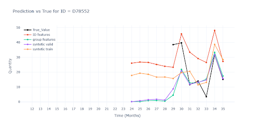
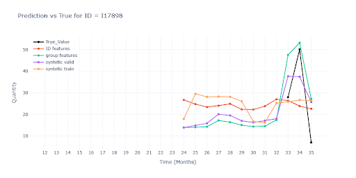
Models shown in the charts:
- 🔴 Red – model with only item-level (ID) features.
- 🟢 Green – model with added group features.
- 🟣 Purple – model with synthetic data applied only during validation.
- 🟠 Orange – model with synthetic data used during both training and validation.
Long sales history of the item
- For items with complete history, the impact of group-features is minimal – the model already has enough information from the item’s own data.
- The benefit of group-level information increases proportionally as history shortens – the fewer own data points, the more important the knowledge of patterns across the group becomes.


Short sales history of the item
- Group-features (🟢 green) keep the level and trend much closer to real sales than the pure ID-model (🔴 red).
- Synthetic data only during validation (🟣 purple) has a similar benefit to pure group-features, but sometimes scales less accurately.
- Training with synthetic data (🟠 orange) more often pulls predictions back toward the group average, suppressing deviations.
No sales history of the item
- Even here, group-features keep the trend and scale much closer to real sales than the red model.
- Without them, the model falls back to the group average, which for some SKUs means dramatic underestimation or overestimation.
- Synthetic data in training can provide a curve shape but loses real variability – results appear “smoothed” and react less to potential fluctuations.
- Overall, predictions for items with no history remain unusable – without a single real sales data point, the model cannot estimate the correct sales scale
Group-features bring the greatest benefit for short histories, where they help keep both trend and scale close to reality. Synthetic data in training, on the other hand, often “smooths out” predictions and reduces variability. Without a single real sales data point, however, predictions remain unusable – the model has nothing to base an accurate sales scale on.