Inventory Forecasting with AI#2

Inventory Forecasting with AI

2. Data Structure & First Pass Analysis

First look at the data

The customer supplied plain text exports — CSV files. Direct integration with internal systems was deliberately postponed; the aim at this stage was simply to verify that an AI model could work on the data.

Each row in the files represents one product in one period and contains:

A unique product identifier (identical in all files)
Seasonality tag, category, type, and segment
Description and any sub-category breakdown
Unit of measure and detailed item description
History for the last 36 months
- Turnover (in units and in currency)
- Quantity ordered
- Dates and labels of promotional campaigns

In total there were roughly 15 000 individual SKUs. The basic time index is the month, which lets us follow sales and inventory development over time.
Even at first glance it was clear the data were incomplete and showed several inconsistencies:

Missing sales history: For many products part or all of the history was absent, typically for new or strongly seasonal items.
Negative sales values: Some records contained negative sales, often returns, cancellations, or input errors.
Unit-of-measure mismatches: Different units make turnover interpretation difficult (pieces vs grams, single units vs thousands).
Duplicate records: Certain items appeared more than once with identical or slightly differing attributes.
Promo duration vs sales granularity: Promotions were recorded in days, whereas sales were monthly.
Uneven history length: Some products had a three-year history; others only a few months.
Other missing data: Absent dates, categories, etc.

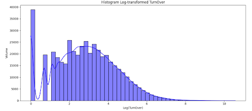
The first graph (box plot) shows the distribution of product turnovers across the entire data-set, plotted on a logarithmic scale, where the second graph (histogram) displays the frequency of individual turnover values.

The median log(turnover) is roughly 3.5, which corresponds to a typical volume of around 33 units per month. Most products fall in the 1.5 – 5 range (≈ 4 – 150 units/month).
A few items, however, exhibit much higher turnovers; these extreme values form the box-plot’s right-hand “tail”.

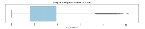
A large share of products has zero or very low sales (left side).
The highest density is between log(turnover) 2 – 4, i.e. roughly 7 – 55 units per month.
Only a small subset lies on the far right—products with very high turnover. They are rare but have a disproportionate impact on total sales volume.

Data Import and Cleaning

Before any forecasting model could be trained, the raw data had to be thoroughly prepared and cleaned. In AI projects this step is often the most time-consuming—and it has a decisive impact on model quality.

Missing sales history
A major issue was incomplete sales history. In some extracts the warehouse system wrote a zero as an empty cell. In others the product did not yet exist for that month, so the field was also empty. To help the model tell the difference, I added a new column –weight- that marks whether the item actually existed in each period.

Negative sales values
Several rows contained negative sales caused by product returns. In agreement with the customer these values were converted to zero to keep the model from being skewed by returns.

Unit-of-measure mismatch
Some items sell only a few pieces per period, while others move by the thousands in the same timeframe. Because a global conversion was not feasible, the model had to learn to scale correctly.

Promo duration vs. monthly sales
Promotions were stored in days and often spanned more months, whereas sales were monthly. I therefore created a column that records the percentage of each month covered by a promo (e.g., promo active 50 % of the month).

Uneven history length
Some SKUs were launched during the 36-month window and had only a short record. To keep a consistent timeline I again relied on the –weight- flag to indicate months before the item existed.
Duplicates and other gaps
Together with the client we removed duplicate rows and filled or dropped remaining missing fields so that the final training set would influence the model as little as possible in a negative way.

Resulting structure

The data were converted into a classic “long” format, where each row represents one product–month combination.
The final data set contains roughly 15 000 SKUs and just over half a million rows.

List of columns:

The list below shows the structure of the prepared long table. In addition to the basic identifiers and commercial attributes, it already includes several auxiliary columns that are essential for modelling—most importantly –weight- and –time_idx-.

ID, seasonality, category, type, segment, unit, name, turnover, price, ordered, date, time_idx, weight, SALE, SALE_INTENSITY

First analyses and patterns discovered

Although the ultimate goal of the project is to forecast inventory levels, a detailed data review showed that it is more practical to predict turnover (expected sales) first. Standard logistics rules (min/max stock, lead times, safety stock) can then convert the sales forecast into an optimal stock target for each month.

Key decisions during data exploration

Some columns were excluded from model training because they do not influence sales volume directly:

Price – in the customer’s setting the selling price showed no clear correlation with quantity sold.
Quantity ordered – supplier performance affects stock, not sales; these variables will therefore be used later, when we translate the sales forecast into stock recommendations.
Segment hierarchy – the “segment” attribute has three levels. To keep the full information I retained all three levels as separate fields: Segment, Segment 1, Segment 2.

Segment	number ID	mean_target	std_target	var_target
AA-BB-UU	91	20.925	44.316	2 001.933
AA-EE-DD	89	54.869	70.83	5 114.107
AA-GG-LL	88	26.011	33.747	1 160.926
AA-AA-SS	89	84.013	173.254	30 598.405
XX-WW-TT	91	50.484	89.99	8 255.076
GG-PP-AA	86	28.943	40.32	1 657.201
DD-GG-VV	85	4.494	5.227	27.855
HH-EE-RR	81	12.802	11.232	128.596
AA-DD-OO	79	21.321	36.809	1 381.121
BB-WW-TT	77	90.052	141.141	20 306.666

Segment2	number ID	mean_target	std_target	var_target
DD	2645	32.412	169.623	29 329.194
FF	2689	119.556	455.99	211 954.269
GG	1687	32.537	67.237	4 608.307
AA	1288	63.001	150.065	22 955.733
BB	611	104.113	287.801	84 433.946
HH	509	84.453	249.227	63 317.309
KK	512	49.896	230.821	54 310.314
OO	471	39.45	102.916	10 796.918
PP	436	56.652	159.096	25 801.689
QQ	339	30.97	84.214	7 229.437

The summary tables list of the ten most common sub-groups in each segment level.
For every sub-group they show number of unique SKUs, average turnover (mean_target), standard deviation (std_target) and variance (var_target).

The overviews reveal that within every segment level there are sub-groups whose sales volumes and variability differ dramatically. A precise segmentation therefore helps the model estimate demand more accurately—even for items with short histories or highly volatile sales.

A similar breakdown was run for the other grouping keys: seasonality, category and product type.

Unit mismatch – One benefit of deep-learning models is their ability to learn not only from a single item’s history but from patterns across the entire assortment. In practice, however, this introduces a scaling challenge: one SKU may sell hundreds of units per month, another only single digits, while a third moves by the thousands.
To prevent such differences from distorting the model, I added a dedicated column—product_volume_bin—that tags every item according to its usual sales volume. With this categorisation the model can separate low-, mid- and high-volume products and handle their relationships more accurately.

Resulting data structure

ID, seasonality, category, type, segment, segment1, segment2, unit, name, turnover, date, time_idx, weight, SALE, SALE_INTENSITY, product_volume_bin

Conclusion & next steps

With the data cleansed and the long table ready, everything looked straightforward—until we tried the first reference models (linear regression, decision trees and friends).

That raised the project’s first real challenge: how to evaluate the forecasts when traditional metrics start to fail? Why this happens and how to solve it will be the focus of the next instalment.