Inventory Forecasting with AI #7

Inventory Forecasting with AI

7. Feature Engineering II – How to Tame Seasonality, Zeros, and Promotions

Seasonal Sales

A classic example: Christmas products. They don’t sell at all for ten months, and then sales suddenly spike in November and December. The key challenge here was teaching the model to distinguish true seasonal demand from random fluctuations or outliers. In the training window (33 months), such items only showed two peaks — which wasn’t enough for the model to recognize a meaningful pattern. As a result, it treated them as noise and continued predicting zeros.

What went wrong:

Too few repetitions – Two peaks in 33 months don’t form a statistically significant sample.
Robust normalization – It softened the spikes, which made it easier for the model to ignore them.
No explicit signal – The model didn’t know that a specific month was special for the given item.

Each visualization includes a chart showing::

Black – Actual historical sales
Red – Model output before adjustment
Green – Model output after adjustment

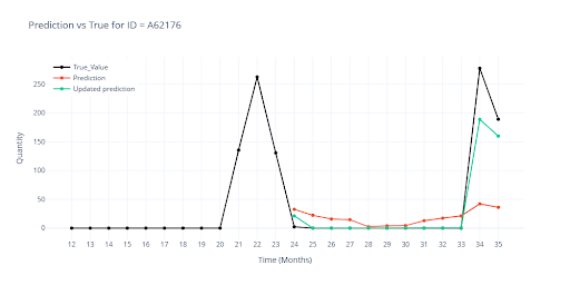
Solution: Feature Engineering to the Rescue

I extended the dataset with new signals to help the model understand seasonality:

Peak is coming – A binary feature that flags the specific month (or time index) when sales consistently spike (e.g., Christmas, Black Friday, summer season).
It’s seasonal – A second binary signal that indicates whether this spike has occurred in at least two consecutive years, helping the model distinguish true seasonality from one-off events.
Average peak size – A numerical feature showing the typical increase in sales during the spike, giving the model a sense of scale.
Maximum peak size – The historically highest recorded spike, useful for anchoring expectations.

Zero Predictions

For part of the catalog, the model consistently predicted zero. Items with very low turnover and long zero-sales stretches quickly “taught” the model a safe rule → Always predict zero.

What went wrong:

Imbalanced signal – The data contained far more zeros than actual sales, so the model naturally slid toward zero predictions.
Missing context: “this is normal” – The model couldn’t recognize that occasional small sales were normal for the item, not noise.
Normalization drowned the signal – Small-volume items got lost among those with high sales, making small variations practically invisible.

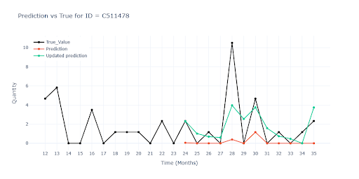
Solution

This turned out to be one of the most difficult challenges. For some items – especially when low volumes were combined with promotional campaigns — zero predictions still dominated.
The breakthrough came only after changing the normalization strategy (individual approach for each feature) and adding new contextual features:

Item age – The model now knows how long the product has been on the market. New items are allowed to have a few initial zeros, while older products with long sales gaps indicate possible decline.
Time since last sale – How many months have passed since the item was last sold. A recent sale increases the likelihood of another one.
Time without sales – How long the item has been inactive. The longer the gap, the more cautiously the model predicts new sales.
Seasonal month flag – A reminder that a seasonal sale historically occurred in this specific month.

Promotional Sales

A typical example is small electronics: most of the year, sales trickle in slowly — just a few units per month. But once the e-shop launches a -20% weekly promo, orders can spike by dozens of units, only to drop back down once the campaign ends. Promotions were fairly common in the dataset — some items had several campaigns per year.

What went wrong:

Promo signal got lost in the crowd – After expanding the dataset with many engineered features, only two were directly related to promotions. Their influence in the model’s attention mechanisms significantly weakened. In other words, in the original dataset, promo indicators were dominant; now they were drowned in noise and largely ignored.
Missing campaign context – The binary SALE feature could say “a discount is active now,” but it didn’t convey how long it lasted or when a similar campaign happened in the past.
Equal treatment of all months – From the loss function’s perspective, underpredicting a promo month was just as bad (or not worse) than underpredicting a regular month.

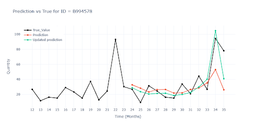
Solution

Once again, I turned to feature engineering and added new contextual information to the dataset:

Time since last promotion – The model learns that the longer the gap since the last promo, the higher the chance that a new one will re-spark demand.
Duration of active promotion – A second signal tells the model how long the current discount has been running.
Product activity – Features such as item age, time gaps between sales, and number of sales in the past year help eliminate false positives for products that have essentially gone inactive.
Discount month indicators – Information about which months in the past the item was typically on sale.

How the Metrics Changed

I reran the test with these new features included. At first glance, global metric changes were minimal, and in some cases, even slightly worse. That’s expected: items with seasonal, promotional, or irregular sales patterns make up only a small portion of the total volume. In the aggregated results, they are outweighed by the rest of the assortment. So the slight worsening likely reflects statistical noise rather than a real drop in model quality. Visual inspection, however, confirmed clear improvements in forecasts for problematic items.

It’s also important to keep in mind that this is a stochastic problem – model outputs naturally vary between training runs. If your setup is correct, these variations should stay small – typically just a few percentage points.

Metrics	Prediction		New prediction
Metrics	Value (ALL)	Value (Item)	Value (ALL)	Value (Item)
WAPE	28.4178	42.0787	29.9001	39.1834
RMSE	46.3156	21.1877	52.8141	20.9628
R²	0.9004		0.9072
MAPE	52.4587		59.802
ROBUST	0.4986	59.7858	0.5259	62.4322
STABLE	0.3677		0.3702