Inventory Forecasting with AI #4

Inventory Forecasting with AI

4. Baseline Models vs. Deep Learning

Why start with classic ML models?

Quick reality check Baseline algorithms train in minutes and instantly reveal major data issues (bad calendar encoding, duplicated rows, etc.).
Reference benchmark Once we know the performance of linear regression or a decision tree, we can quantify exactly how much a deep-learning model must improve to justify its higher cost.
Transparency Simpler models are easier to explain; they help us understand the relationship between inputs and outputs before deploying a more complex architecture.

Baseline Models	How They Work
LR – Linear Regression	Can capture simple increasing/decreasing trends. Once the data becomes more complex, it quickly loses accuracy.
DT – Decision Tree	Can handle more complex curves and nonlinearities, but if the tree grows too deep, it becomes overfitted – it starts repeating patterns.
FR – Random Forest	Averages out errors from individual trees → more stable than a single tree, but more memory-intensive and slower when dealing with a large number of items.
XGB – XGBoost Regressor	Often the best among traditional ML models – it can capture complex relationships without much manual tuning.
GBR – Gradient Boosting Regressor	Good as a low-cost benchmark: if even this fails, the data is truly challenging.

What Does a 12-Month Forecast Visualization for 4 SKU Look Like?

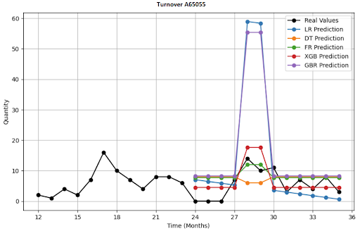
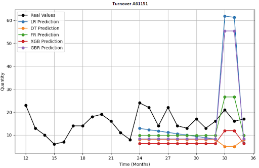
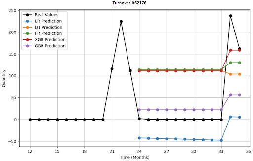
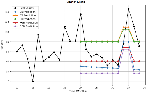
Deep Learning (DL) Architectures I Deployed

For comparison, I built three basic deep learning models. In all cases, these are AI models designed for time series forecasting. While the baseline models belonged to the simpler category, these belong to the more complex end of the spectrum.

DL algoritmus	How It Works	Advantages / Disadvantages
DeepAR (Autoregressive LSTM)	Learns from similar items; during prediction, it generates the full probabilistic range of demand → we can see both optimistic and pessimistic sales scenarios.	For new products, long-tail items, or series with many zeros and extremes, it tends to "smooth out" the curve.
TFT (Temporal Fusion Transformer)	Excellent for complex scenarios – it automatically selects which information is important and can explain its choices.	Best for complex datasets with many external signals, but requires a large amount of data and has long training times.
N-HiTS (Hierarchical Interpolation)	Decomposes a time series into multiple temporal levels (year/month/week), applies a dedicated small network at each level, then recombines them.	Great for long forecast horizons and fast inference, but requires a regular time step.

Why These Complex Models?

They capture subtle and long-term seasonal patterns and promotional effects that classical ML often overlooks.
They share learned knowledge across the product range — helping new items and those with short histories.
They return uncertainty intervals, so the buyer receives a recommendation of “how much to order in both optimistic and pessimistic scenarios.”

What Does a 12-Month Forecast Visualization of DL models for 4 SKU Look Like?

Results

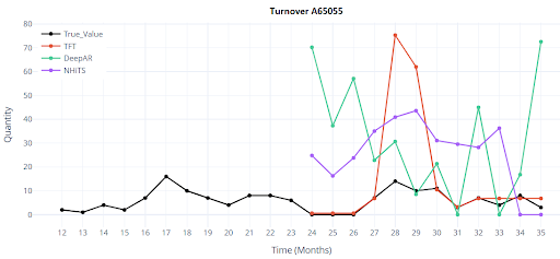
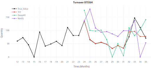
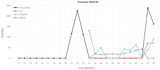
The testing was conducted only under Scenario 1 — both training and validation were performed on the same dataset. I used 5,000 products with a full 36-month history.

Classical models provide an initial orientation, but even the best of them fall short of the target accuracy. Deep learning brings a significant improvement — even in the basic configuration, it reduces the error by half or even two-thirds. This is a clear signal that it’s worth investing time into tuning features, hyperparameters, and deploying the model in production.

Comparison metrics between ML and DL models. I started using advanced validation metrics only at a later stage.

ML - baseline models
Metrics	R²	WAPE	RMSE	MAPE
GBR	0.4259	124.9833	173.599	275.8702
FR	0.3444	133.5684	157.6839	217.063
DT	0.2529	142.5767	165.8517	212.5132
XGB	0.2153	146.125	168.5045	266.1286
LR	0.0745	158.6966	200.3072	477.9817

DeepLearning models
Metrics	R²	WAPE	RMSE	MAPE
DeepAR	0.847	53.615	62.8242	188.5804
TFT	0.3901	30.2255	125.4162	141.6336
NHiTS	0.432	206.9327	121.0321	382.6455

Test 2 – Encoder vs Decoder

In the previous phase, I confirmed that deeper (DL) architectures clearly outperform traditional ML. Before diving into tuning parameters like loss function, optimizer, or dropout (which I won’t cover here), it’s essential to understand the encoder–decoder architecture. In time series models, this is a key component that determines how much of the past the model “reads” and how far into the future it predicts.

Encoder: Defines how much of the historical data the model uses to generate a single prediction. You can think of it like a buyer looking at the last 12 months of history.
Decoder: Represents the forward-looking part – it generates predictions based on the information provided by the encoder.

Unlike a human buyer, the architecture creates multiple predictions (sliding windows) during training for each product. If I have 36 months of history, and I want the model to look back at the last 18 months and predict the next 3 months, then 18 sliding windows are generated during training over this time range.

Encoder	Decoder
0-18	19-21
1-19	20-22
...	...
17-35	36-38

A three-year history thus creates 18 training scenarios for each item; the model sees all possible transitions (e.g., winter → spring, Christmas → January, etc.).

Main difference and impact on model behavior:
What’s the difference between setting the encoder length to 18 versus 30 months?
The key difference lies in the types of patterns the model learns and what it emphasizes.
It’s a classic trade-off between flexibility and stability.

Encoder_length = 18	Encoder_length = 30
Better adaptation to changes: model reacts faster to sudden market shifts (trend, promotion)	Good in seasonality and long-term trends: Better in captures repeating patterns and slow long-term trends
More training windows: Faster learning, lower risk of overfitting (especially for short histories)	Prediction stability: Robust against short-term noise
Lower memory and computation requirements: Faster inference and training	Fewer training windows: Longer training, higher overfitting risk if data is limited
Struggles with seasonal cycles: The model may not fully learn patterns that repeat over multiple years	Slower reaction to changes: Takes longer to adapt to sudden market shifts (trends, promotions)
Seasonal memory: Higher risk of "forgetting" past seasonal peaks like Christmas.	Higher memory and computation requirements

How to Choose?

There’s no universally best setting. In practice, I tested encoder lengths of 12 / 18 / 24 / 30 months, and the most balanced turned out to be encoder = 18 months, decoder = 3 months.
It provides enough historical context, generates a large number of training windows, and responds well to short-term market changes.