In the previous article, I worked with a dataset where the main challenges were seasonality and promotional events. These factors negatively affected simpler models while highlighting the advantages of more complex approaches that were better able to capture changes over time.
The second project addresses a fundamentally different type of problem. Unlike the first project, the challenge here is not the lack of historical data, but the fact that most of the data contains no information at all. The model is not only predicting sales volume, but primarily whether a sale will occur in the first place. This has a direct impact on planning — forecasting errors here do not simply mean lower accuracy, but either unnecessarily held inventory or unavailable products.
As a result, the forecasting problem naturally splits into two parts:
This distinction fundamentally changes both the behavior of the models and the way their performance must be evaluated.
The dataset contains weekly sales data for approximately 5,000 products over a three-year period.
The differences are also visible in sales volumes:
The basic characteristics of the dataset are summarized in the following table:
| Parameter | Value |
|---|---|
| Number of products | 5 000 |
| Data frequency | Weekly |
| Longest history | 161 weeks |
| Shortest history | 2 weeks |
| Share of periods 1–6 months | 1.7% |
| Share of periods 7–12 months | 2.3% |
| Share of periods 13–24 months | 13.1% |
| Share of periods 24+ months | 92.8% |
| Average sales volume | 38.2 |
| Average sales volume (without zero values) | 89.4 |
| Median sales volume (without zero values) | 5.0 |
| Maximum sales volume | 63 400 |
| Share of zero sales | 57.3% |
From a demand planning perspective, this represents a less typical but highly important scenario — especially for slow-moving products. For easier comparison, the results in the charts are presented in monthly form despite the dataset using weekly frequency.
As in the previous project, the experiments were performed on subsets of the dataset divided according to the history length of individual products.
The reason is straightforward — historical depth has a major impact on forecast quality.
Each of these scenarios represents a different challenge, and their combination with a high proportion of zero sales significantly affects the behavior of the individual models.
The same validation strategy as in the previous project was used to compare the individual approaches. Models were trained on historical data and evaluated on the following time period. This setup reflects real-world usage, where future demand is predicted based on past observations.
However, for this dataset it is necessary to evaluate two aspects simultaneously:
The evaluation metric therefore combines both perspectives — penalizing both inaccurate quantity predictions and incorrect predictions of zero-sales periods.
The resulting value represents the overall prediction error — the lower the value, the more accurate the forecast. However, the results must always be interpreted in the context of individual scenarios, since the differences between models manifest differently here compared to the previous project.
Through analysis of the dataset, I identified that the primary challenge is the high proportion of zero sales. To interpret the charts correctly, it is useful to focus on several key aspects:
It is precisely the combination of these factors that determines how difficult forecasting a particular product becomes. Let us now look at several concrete examples of how this data behaves in practice.
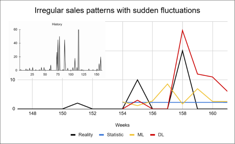
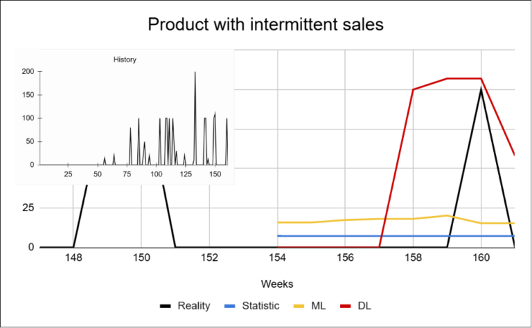
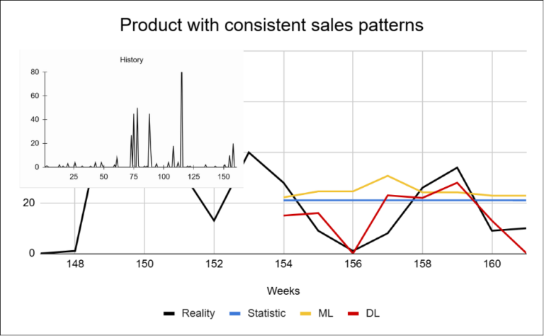
These examples show that the challenge of sparse data is not limited to the high proportion of zero-sales periods alone. Individual products differ not only in how frequently they are sold, but also in sales volume and in how stable their behavior is over time. In sparse datasets, the key challenge is therefore not only the magnitude of the forecasting error, but whether the model can correctly predict the occurrence of a sale itself.
These differences are subsequently reflected in the model results. Let us now examine how the individual approaches performed across the different scenarios.
After understanding the nature of the data, we can examine how the individual approaches performed in practice. As in the previous project, the results were evaluated according to product history length. Unlike the first project, the differences between approaches in this case are significant across all scenarios. Deep learning achieved the best results in every scenario, maintaining a relatively consistent margin over the other approaches. On average, it reduced forecasting error by more than 50% compared to statistical methods and by approximately 40% compared to machine learning.
The reason lies in the nature of the dataset itself. The high proportion of zero-sales periods combined with highly irregular product behavior creates an environment where simpler models struggle to effectively capture the underlying data structure. Statistical methods and Machine learning approaches tend to simplify reality — often converging toward the mean or generating overly stable forecasts that fail to reflect the actual behavior of the data. Deep learning performs better in this scenario primarily because of its ability to leverage information across the entire product portfolio and capture at least part of the hidden patterns present in the data. The exception is newly introduced products (1–5 months), where the differences between approaches become smaller.
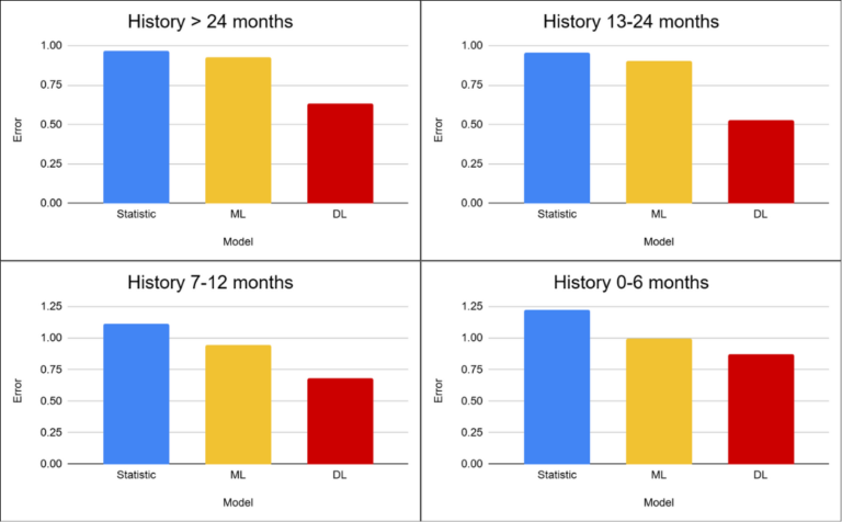
In this scenario, the key challenge is the lack of data combined with a higher degree of randomness. Forecasts are generally less reliable here regardless of the selected approach.
As a result, the main question in this project is no longer the choice of model itself. The critical factor is the ability to handle irregular behavior and a high proportion of zero values.
This dataset highlights a fundamentally different problem compared to the previous project — the challenge is not the complexity of patterns, but the existence of sales themselves. The high proportion of zero values significantly changes the nature of forecasting: the models are not only predicting quantity, but primarily whether a sale will occur at all.
Statistical methods and machine learning approaches tend to simplify the behavior of the data and revert toward the mean. Deep learning achieves better results in this scenario mainly because of its ability to leverage information across the entire portfolio and capture at least some of the hidden patterns within the data.
At the same time, it is important to set realistic expectations correctly. For this type of data, it is not realistic to expect highly accurate forecasts for individual periods, even from advanced models. Sales occur irregularly and often without a clear pattern. Without sufficient historical data and under such a high degree of variability, it is practically impossible to reliably predict exactly when a sale will occur and in what quantity. However, this does not mean that forecasting has no value.
The value of the model in this case is not precise prediction of individual weeks, but rather its ability to reduce uncertainty in the planning process.
In the next article, we will examine a third type of dataset that combines multiple dimensions and introduces another layer of complexity.
IČO: 172 28 018
DIČ: CZ 172 28 018
Data Box ID: ykwdnxf
sales@neebile.cz
Jičínská 226/17, Praha, Žižkov, PSČ 130 00 Česká republika
(910) 658-2992
© 2025 Vytvořeno DigitalWays