This article is based on a personal project and practical testing on real-world inventory forecasting data. It represents the author’s private initiative, and the conclusions presented do not reflect the position of any company. In the previous projects, I worked with datasets where the main challenge was either limited historical data or a high proportion of zero sales. The third project focuses on a different type of scenario. The dataset contains daily sales data with sufficiently long historical coverage for all products.
The primary challenge here is not missing data, but external factors that systematically distort sales behavior — particularly weekends, holidays, and differences between locations. Without correctly interpreting these effects, even more advanced approaches begin to fail. The model is therefore not solving a lack of data problem, but rather the ability to understand why the data changes over time.
The dataset contains daily sales data for approximately 1,800 combinations over a period of 4.5 years.
The differences are also visible in sales volumes:
The basic characteristics of the dataset are summarized in the following table:
| Parameter | Value |
|---|---|
| Number of combinations (group/location) | 1 800 |
| Data frequency | days |
| Longest history | 1 688 days |
| Shortest history | 118 days |
| Share of periods 1–6 months | 1.9% |
| Share of periods 7–12 months | 0.0% |
| Share of periods 13–24 months | 3.7% |
| Share of periods 24+ months | 94.4% |
| Average sales volume | 383.7 |
| Median sales volume | 16.0 |
| Maximum sales volume | 31 024 |
| Share of zero sales | 26.0% |
At first glance, the dataset does not appear to be extremely complex. Most products have a long historical record, and zero-sales periods account for approximately one quarter of the data. It is precisely the combination of stable historical data and external influences that creates an interesting forecasting scenario — simpler models have enough data available, but may still struggle to correctly respond to changes caused by calendar effects or location-specific behavior.
To compare the individual approaches, the same validation strategy as in the first project was used. Models were trained on historical data and evaluated on the following time period.
Unlike the previous projects, the primary challenge here is neither limited historical data nor an extreme proportion of zero values. Instead, the model must correctly respond to external influences such as holidays or location-specific effects. If these factors are ignored, they lead to systematic planning errors — for example, consistently underestimating or overestimating demand.
The key factors are:
Based on the nature of the dataset, I expected the differences between models to be smaller than in the previous projects. However, approaches capable of utilizing external input features were expected to have an advantage.
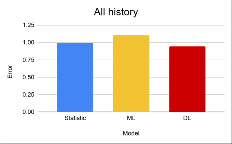
The results show that the differences between approaches are relatively small in this scenario. Deep learning achieves the best performance, with an improvement of approximately 5%. The main reason is its ability to utilize external inputs such as holidays or location-specific information.
Statistical methods perform surprisingly well because the dataset contains stable historical data and strong seasonal patterns. More unexpected are the weaker results of machine learning approaches, where I would have expected performance at least comparable to statistical models, if not better. One possible explanation is the limited ability of these models to handle complex combinations of calendar-related and location-specific factors.
A difference of approximately 5% is significantly smaller than in the previous projects, where the gaps reached tens of percent. This confirms that for stable datasets with sufficient historical depth, the choice of model becomes a less critical factor.
Although the aggregate metrics show very similar results across models, a more detailed view of individual products reveals partially different behavior patterns.
Simpler models tend to pull predictions toward the mean. In datasets with a higher proportion of non-zero values, this issue is often hidden within aggregate evaluation metrics. Deep learning, on the other hand, responds more effectively to short-term changes and is better able to capture fluctuations that are important for planning.
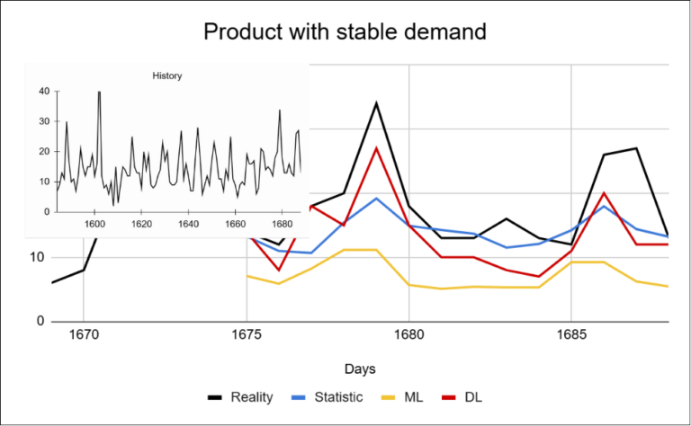
For stable products with a growing trend, all approaches perform relatively well.
The main differences can be seen in how the models react to fluctuations:
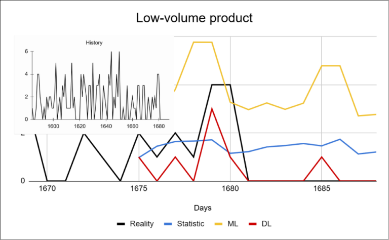
For low-volume products, the differences between models become more significant. The reason is the high proportion of zero or very small values, which pushes predictions toward the mean. Simpler models struggle to correctly estimate the occurrence of sales.
In this project, deep learning does not explicitly predict the probability of a sale occurring (as in Project 2), but it is still better able to capture changes in sales volume.
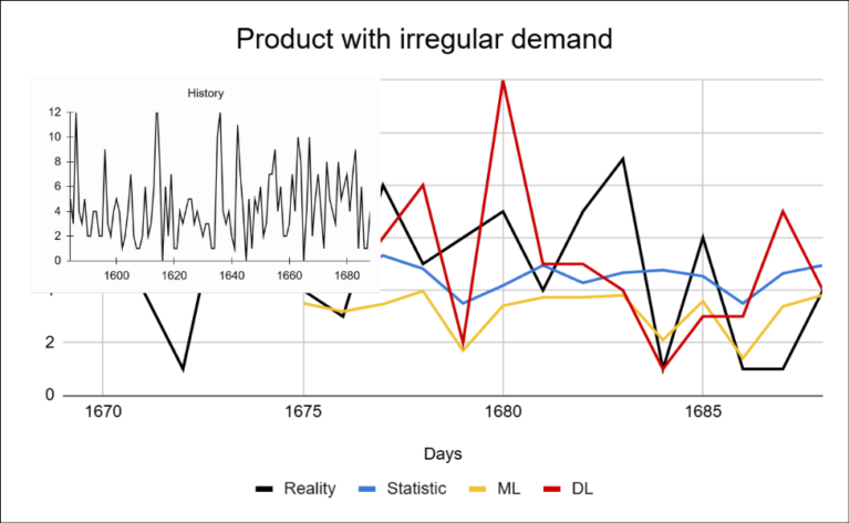
For irregular products, the accuracy of all models decreases. Simpler approaches tend to stabilize predictions around the mean, which results in the loss of information about the actual behavior of the data. Deep learning is able to react more effectively to changes, but even here stable and highly accurate forecasts cannot be expected.
Aggregate metrics indicate only minimal differences between the models. However, when examining individual products, the reality looks quite different. Extreme forecasting errors can easily disappear within aggregate metrics. A model that fails on a smaller subset of products may appear equally effective on average as a model that behaves more consistently.
When the evaluation focuses only on specific products, the differences between approaches become significantly larger. This means that even when aggregate results appear similar, the practical impact of the models can differ substantially — especially for key products or during periods of abnormal fluctuations.
Compared to the previous projects, this scenario highlights a different type of challenge. While the earlier projects were primarily affected by data availability or data structure, the key factor here is the model’s ability to correctly interpret external influences.
In this project, the data is relatively stable and well-structured. As a result, the differences between models are much smaller than in the previous scenarios. Statistical approaches achieve surprisingly strong results. The main challenge here is not data availability, but the ability of the model to react appropriately to changes over time.
However, a more detailed analysis reveals that simpler models fail on specific products, especially during fluctuations. Thanks to their ability to incorporate external inputs, deep learning approaches are better able to capture the underlying structure of the data and respond to changes. In practice, this means a more precise response to changes that can directly affect inventory levels.
The key question is therefore not which model is objectively the best, but whether the improvement in forecasting accuracy justifies the additional complexity of the solution.
In the next article, we will evaluate the individual projects and examine whether — and how — advanced deep learning models can be used without a dedicated implementation team.
IČO: 172 28 018
DIČ: CZ 172 28 018
Data Box ID: ykwdnxf
sales@neebile.cz
Jičínská 226/17, Praha, Žižkov, PSČ 130 00 Česká republika
(910) 658-2992
© 2025 Vytvořeno DigitalWays