#1. Forecasting in Practice

Forecasting in Practice

1. Does AI Make Sense for Smaller Companies?

Current State – Simple Planning

Most companies outside large enterprises still plan demand the same way they did years ago – using Excel, simple models, and human experience.

It works for a while. The problem appears when reality becomes more complex. Seasonality changes, promotions distort demand, new products have no history, and knowledge often exists only in people’s heads – people who eventually leave. The result? Inaccurate forecasts, excess inventory, or stockouts.

Today’s landscape is heavily influenced by AI, especially LLMs. It is often claimed that these models will transform forecasting just as they transformed text processing or programming.

But is that really the case?

LLMs work extremely well with text, interpretation, and data analysis. However, time series forecasting is a different type of problem. It requires models that understand temporal dependencies, seasonality, and data structure.

So the question is not whether to use AI. The question is how to use it correctly – and which approach makes sense in real-world environments.

That is exactly what this article focuses on. Based on real data, I compare statistics, machine learning, and deep learning – showing where each approach works, where it fails, and what it means in practice.

And most importantly – whether advanced models make sense even for smaller companies.

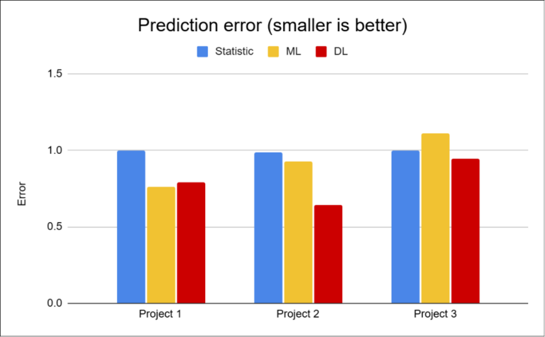
Real Data – “Three Different Worlds, One Problem”

Before looking at the approaches themselves, it is important to understand the data. In practice, there is no such thing as a “typical” problem. Every dataset has its own characteristics, which strongly influence model performance. Projects Used in Testing:

Project 1

15,000 products
48 months of history
sales forecasting
mix of seasonality, promotions, irregular sales

Project 2

7,000 products
36 months of weekly data
sales forecasting
~75% zero values

Project 3

54 stores, 33 categories
60 months of daily data
revenue forecasting
https://www.kaggle.com/competitions/store-sales-time-series-forecasting

Key Challenges

Factors that significantly impact forecasting quality:

Seasonality – not only recurring patterns, but also how they evolve over time. What worked last year may not apply this year.
Promotions – they can temporarily boost sales, but at the same time disrupt normal behavior patterns. The challenge is distinguishing long-term trends from one-off effects.
Sparse data – a high number of zero sales represents one of the biggest challenges. Models naturally tend to push predictions downward because they learn that zero is often the “correct” value.
Noise in data – errors, fluctuations, one-off events, or external influences. When sales lack a clear pattern, it becomes difficult for models to distinguish real signal from random variation.

These factors determine which model will succeed – and which will fail.

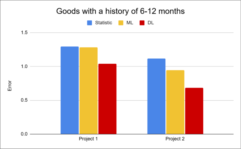
Alongside data characteristics, the length of history also proved to be a critical factor. Products with long histories tend to behave relatively stable, while new or short-lived items are significantly harder to forecast.
More data does not automatically mean better predictions. Longer histories often include more noise and irregularities, which can make learning more difficult for models.

Hypothesis

The core hypothesis was simple:

For stable data, complex solutions often do not make sense – the accuracy gain is small and does not justify higher costs
As data complexity increases, the impact of errors grows – and so does the value of advanced models

Experiment Methodology

Three approaches were compared:

Statistical methods are among the simplest approaches. They are based on the assumption that future behavior can be derived from historical patterns. They are fast, cost-effective, and easy to implement.
Machine learning models look for deeper relationships between inputs and outputs instead of describing the series with a single equation. They handle non-linearity, are more robust to noise than statistical methods, and remain relatively easy to deploy.
Deep learning models can learn temporal behavior directly from data. They capture complex non-linear dependencies and can incorporate multiple inputs such as promotions, product groups, and other contextual features. The downside is higher complexity and computational requirements.

For comparison, a unified validation strategy was used. Models were trained on historical data, with the last six periods reserved for validation. Each approach was optimized independently to achieve the best possible performance within its respective setup.

Results

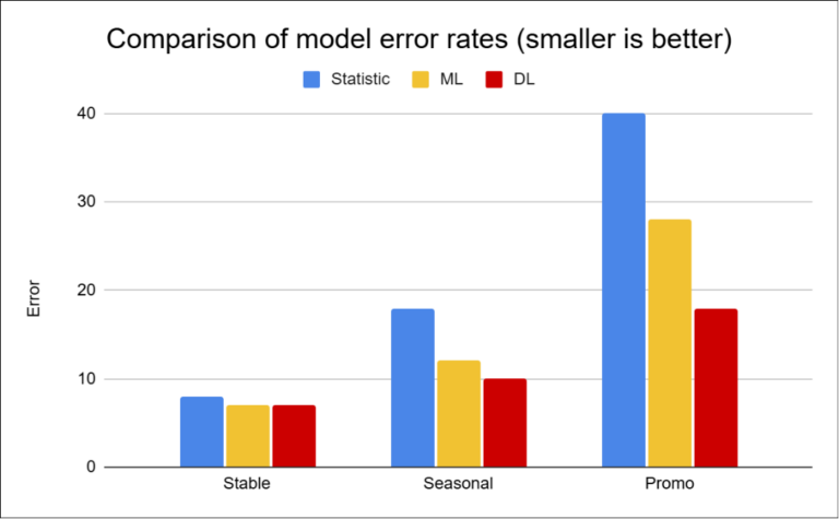
Real-world datasets are rarely clean. They usually combine stable, seasonal, and irregular sales, along with noise and short histories.

The results show a clear pattern:

For stable products, simple models are often sufficient — the added value of more complex solutions is minimal and does not justify their cost and complexity.
For seasonal products, however, the differences between approaches start to have a real impact on inventory levels and product availability. Both machine learning and deep learning bring measurable improvements.
For irregular or promotional products, especially with a short history, the differences are the most significant – deep learning clearly outperforms the other approaches.

Project 2 shows that datasets with a high number of zero and irregular sales represent a major challenge for traditional approaches.

In contrast, Project 3 demonstrates that in more stable scenarios, simpler methods can be sufficient.

However, this changes significantly for items with shorter history. It is precisely in these cases that the differences between approaches become most apparent — simple models lose accuracy, while deep learning often manages to maintain significantly better performance.

The difference between models is not just about percentages. It is about how much inventory you hold — and how many customers you lose. The following overview shows the business impact of different approaches based on the tested scenarios:

Product Type	Improvement	Inventory Impact	Stockout Impact
Stable	1–3 %	Minimal	None
Seasonal	8–12 %	inventory reduction 3–5 %	Fewer stockouts
Promo / Irregular	20–40 %	inventory reduction 10–20 %	Fewer stockouts, higher revenue

These values are based on tested scenarios and practical experience. Model selection should therefore not be universal, but depend on the characteristics of a specific part of the portfolio. In practice, this means that different types of products require different approaches. While stable items with long history can be effectively forecasted using simpler methods, seasonal, irregular, or new products expose the limits of these approaches — and the value of more complex models increases significantly.

The key is not to find one “best” model, but to choose the right approach for a specific type of problem.

Conclusion

The results show when each approach makes sense.

Statistical methods work well when data is stable and predictable.
Machine learning brings improvement in more complex scenarios. Typically, these are situations where deviations start to appear and lead to worse planning decisions.
Deep learning delivers the most value when seasonality, irregularity, and multiple influencing factors combine. These are exactly the situations where the biggest planning errors occur — excess inventory or, on the other hand, out-of-stock situations.

The difference between approaches is not just visible in metrics, but in how much capital you hold in inventory and how many orders you fail to fulfill.

Deep learning is often not used in practice because every change requires intervention in the solution — which means additional time and cost. However, once you introduce a unifying layer over this process, the way of working changes fundamentally. Instead of making major changes to the solution, you adjust parameters and systematically test different variants. This can reduce development time from months to weeks.

The more complex and less predictable the data, the bigger the difference between approaches — and the more sense it makes to use deep learning. At the same time, without proper setup, its real-world impact can be close to zero.

In the following articles, I will focus on specific projects and show how different approaches behave in practice. In the final part of the series, I will break down the metrics, model setup, and practical implementation experience in more detail.