Inventory Forecasting with AI #8

Inventory Forecasting with AI #

8. Generalization – Including Items with Incomplete History

Full Dataset Test

In the previous chapter, we confirmed that the model performs “flawlessly” for the 70% of the assortment with a complete 36-month history.
Now it’s time for a real challenge: what happens when we unleash the model on the entire dataset, including products with shorter or even nonexistent history?

History Length	Number of Items	Share of Assortment
36 months (full history)	10105	70.00%
12–35 months	2668	18.00%
Less than 12 months	1211	8.00%
No history	519	4.00%

All the following experiments use the same model I built in earlier chapters – i.e. including all feature engineering improvements and outlier control. I’m still using Scenario 2: 33 months for training, 3 months for validation.

I tested three training variants, while always validating on the full dataset:

Variant	Training Includes	New Items in Validation
A – Full history	Only items with complete history	468
B – Min. 1 month	All SKUs with at least 1 historical data point	73
C – No restrictions	All items, including those with no historical data	0

Poznámka: Například ve variantě Plná historie (A) bylo při validaci nalezeno 468 nových položek, které model při tréninku neviděl.

What I’m Analyzing

Global performance metrics (R², WAPE, RMSE, etc.) across variants A, B, and C
Impact on items with full history – Does adding “data-poor” items hurt performance on well-covered SKUs?
Behavior of new or short-history items – Can the model transfer knowledge from long time series, or do predictions still collapse to zero or behave randomly?

Metrics	Full history		Any history		1 months min history
Metrics	Value (ALL)	Value (Item)	Value (ALL)	Value (Item)	Value (ALL)	Value (Item)
WAPE	41.0748	133.7093	38.4147	93.4879	34.6338	58.0287
RMSE	48.8867	24.5721	57.3472	23.2029	35.4181	18.5031
R²	0.7952		0.7408		0.8511
MAPE	131.7516		70.8846		68.2377
ROBUST	0.4741	158.7209	0.4785	78.5382	0.5312	77.5052
STABLE	0.5013		0.4613		0.3681

Summary of Results

Training on full-history SKUs only (left column): Every SKU used in training had a complete 36-month history. However, the model failed dramatically when asked to predict new or unseen SKU – with Item-level WAPE and MAPE both exceeding 130%.
Training on all SKUs, including those with zero history (middle column): This variant did not improve global metrics and actually increased RMSE. Including completely unknown products in training added significant noise to the learning process.
The optimal variant was training on all items with at least 1 month of history (right column): This approach substantially reduced prediction error while maintaining a strong R² score. I selected this configuration as my new baseline for further development.

Visual Inspection

As in previous chapters, I manually reviewed forecasts for several problematic SKUs – this time expanded to include items with short or no history.

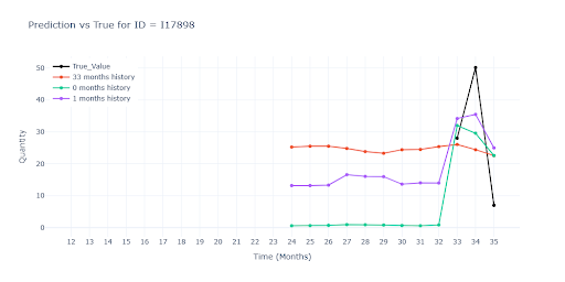
Displayed model:

🔴 Red – Model trained on full-history items only
🟢 Green – Model trained with items including zero-history
🟣 Purple – Model trained on items with at least 1 month of history

Note: To maintain context on each item’s history length, all plots show the full 36-month window.

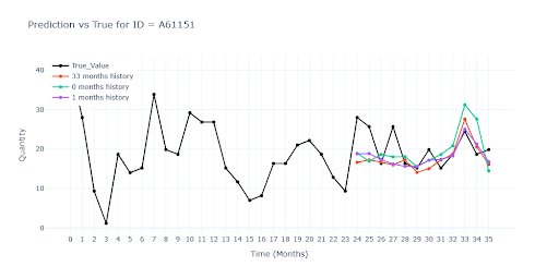
For items with full history, all three models produced nearly identical forecasts. This means that even when items with missing history are added to training, the model remains stable – thanks to the weight feature, it learns to skip empty periods without distorting the signal.

Interestingly, models trained on mixed-history items (especially the purple one) often predicted higher and more accurate seasonal peaks than the model trained solely on complete series. Shorter time series likely provided extra contextual signals that helped the network generalize seasonal patterns more boldly – and, in many cases, more accurately.

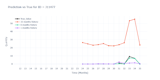
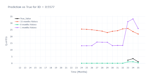
For items with partial history, the red model (trained only on full-history data) performed significantly worse. Since it had no access to a single real record for these SKUs during training, it had no understanding of their typical turnover. As a result, the model could only guess based on similarity to other products — often leading to inaccurate predictions.

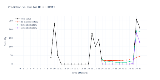
We see a similar drop in performance for items with very short history. Once again, the red model had nothing to grab onto – no useful data to estimate demand. The other two models, while also working with limited history, were still able to estimate the item’s turnover level and get much closer to reality.

In the second visual, you can clearly see how the green and purple models successfully “pull up” the prediction based on similar SKUs. Even without direct historical data, they predict a sales spike in the second month, simply because similar products in the same group show the same pattern. In other words, the model correctly transferred knowledge from richer time series instead of defaulting to zero.

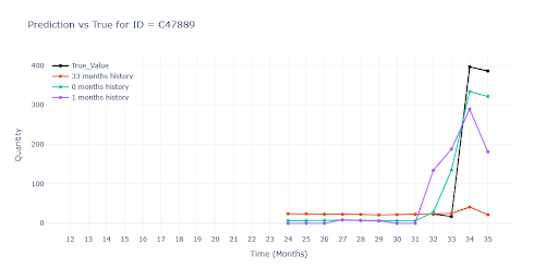
When no historical data is available at all, predictions become little more than educated guesses into the void. Without a real sales anchor, the models default to some kind of segment average – which leads to significant underestimation for some items and overestimation for others. Without at least one actual sales data point, the forecast remains highly uncertain and difficult to interpret.

How Model Performance Varies by History Length

To get a more detailed view, I validated performance across five different scenarios, grouped by the length of each item’s history. The following insights are based solely on the model trained with items that had at least one month of sales history (green line in previous charts).

Metrics	Full dataset 100% items		36 months 72% items		12-35 months 18% items
Metrics	Value (ALL)	Value (Item)	Value (ALL)	Value (Item)	Value (ALL)	Value (Item)
WAPE	34.6338	58.0287	33.4331	45.3934	36.5081	49.183
RMSE	35.4181	18.5031	38.1581	19.3561	23.4648	13.58
R²	0.8511		0.8535		0.7525
MAPE	68.2377		61.9222		67.8013
ROBUST	0.5312	77.5052	0.5282	62.6903	0.5365	66.6689
STABLE	0.3681		0.3505		0.4093

Metrics	6-12 months 4% items		1-6 months 4% items		No history 2% items
Metrics	Value (ALL)	Value (Item)	Value (ALL)	Value (Item)	Value (ALL)	Value (Item)
WAPE	37.7617	55.3109	56.1651	61.0081	117.1288	884.835
RMSE	36.3108	11.9183	46.4892	34.9088	45.6377	33.9161
R²	0.7767		0.5277		-0.0826
MAPE	69.1417		98.2678		636.876
ROBUST	0.5478	69.4062	0.5247	105.5108	0.4238	940.0516
STABLE	0.4296		0.5151		1.3529

Key Takeaways:

Stable metrics across history buckets – The model performs consistently well up to the 6–12 month category. This shows it can handle incomplete history quite effectively. The only notable drop is in R², which is expected due to the lack of historical variance.
Lower RMSE in 12–35 and 6–12 month groups – These items tend to have moderate turnover, so absolute prediction errors are smaller, which brings down RMSE.
Short histories (less than 6 months) – Performance begins to degrade here. The model lacks a sense of typical turnover, and must rely more heavily on similarity with other items. Errors grow quickly — but still remain within reasonable bounds.
Zero history – Metrics are heavily skewed. The model uses group-level signals, but lacks any concrete context for the individual SKU, resulting in unstable outputs.

Mission: „Short-History Items“

It became clear that I needed to focus primarily on SKUs with short histories. For brand-new products, with no sales records and no signal about typical volume, the model simply cannot guess effectively. That’s why I set a practical minimum requirement: At least one real month of sales history. From this single data point, the model can infer an approximate scale of demand – and then reconstruct the rest of the pattern from similar items using group relationships and embedding vectors.

To achieve this, I began testing two approaches:

Group-level features – Every SKU belongs to a group and receives its own embedding vector. I aim to enrich this with explicit signals from the group, such as average turnover, seasonal shape of the group, etc.
Synthetic history – For new items, I generate a “warm-up” period: the first few months are filled in using estimates based on similar SKUs. These synthetic data points are used only for feature calculation — this gives the model a rough idea of the curve shape (trend, seasonality) without affecting the training of target values.